K-Nearest Neighbors & Random Forest: Classification of UCI Glass & Wine Datasets
Project Overview
This project involved implementing and comparing K-Nearest Neighbors (KNN) and Random Forest classification methods on the UCI Glass and Wine datasets. The analysis focused on exploring the impact of different parameters on model performance, comparing classification accuracy across methods, and identifying the most important features for classification. The workflow covered data exploration, preprocessing, model training with cross-validation, hyperparameter tuning, and comprehensive performance evaluation.
Date: 2025-03-07
Methodology
The analysis followed a structured approach to model building and evaluation:
- Dataset Loading & Exploration: Loaded the UCI Glass and Wine datasets, examined their structure, checked for missing values, and analyzed class distributions.
- Data Preprocessing: Standardized all features to ensure fair comparison across variables with different scales. Performed preliminary feature correlation analysis.
- KNN Implementation: Applied the K-Nearest Neighbors algorithm with different k values (1-30). Used cross-validation to find the optimal k for each dataset.
- Random Forest Implementation: Trained Random Forest models with varying mtry parameters (number of variables randomly sampled at each split). Optimized the number of trees and node size.
- Feature Importance Analysis: Extracted and visualized feature importance from the Random Forest models to identify the most significant predictors for classification.
- Performance Evaluation: Compared models using accuracy, confusion matrices, precision, recall, and F1-scores. Analyzed misclassification patterns.
- Ensemble Approach: Explored combining KNN and Random Forest predictions for potentially improved performance.
Key Findings
- Optimal KNN Parameters: For the Glass dataset, k=1 provided the highest accuracy (70.1%), while for the Wine dataset, k=5 was optimal (97.8%). This suggests the Wine dataset has more well-defined, clustered classes.
- Random Forest Performance: Random Forest outperformed KNN on the Glass dataset (76.2% vs. 70.1%) but performed similarly on the Wine dataset (97.8%). This indicates that ensemble methods handle complex, noisy data better.
- Feature Importance: For Glass classification, refractive index, magnesium, and aluminum content were the most significant features. For Wine, alcohol content, flavonoids, and color intensity were most predictive.
- Parameter Sensitivity: KNN performance was more sensitive to parameter changes (k value) than Random Forest. This suggests Random Forest is more robust and requires less fine-tuning.
- Class Imbalance Effects: In the Glass dataset, classes with fewer samples had lower classification accuracy, highlighting the importance of addressing class imbalance in real-world applications.
- Cross-Validation Benefit: Cross-validation significantly improved the reliability of the model performance estimates, especially for the smaller Wine dataset.
Implementation Details
Data Loading and Preprocessing
# Load necessary libraries
library(class)
library(randomForest)
library(caret)
library(e1071)

# Load UCI Glass dataset
data(Glass, package = "mlbench")
str(Glass)
summary(Glass)

# Load UCI Wine dataset
data(wine, package = "rattle")
str(wine)
summary(wine)

# Check for missing values
sum(is.na(Glass))
sum(is.na(wine))

# Standardize features for both datasets
glass_std <- as.data.frame(scale(Glass[, -10]))  # Exclude Type column
glass_std$Type <- Glass$Type

wine_std <- as.data.frame(scale(wine[, -1]))  # Exclude Type column
wine_std$Type <- wine$Type
KNN Implementation with Cross-Validation
# Function to perform k-fold cross-validation for KNN
knn_cv <- function(data, target_col, k_value, folds = 10) {
  # Create folds
  set.seed(123)
  fold_indices <- createFolds(data[[target_col]], k = folds)

  # Initialize accuracy vector
  accuracies <- numeric(folds)

  # Perform cross-validation
  for (i in 1:folds) {
    # Split data
    test_indices <- fold_indices[[i]]
    train_data <- data[-test_indices, -which(names(data) == target_col)]
    test_data <- data[test_indices, -which(names(data) == target_col)]
    train_labels <- data[-test_indices, target_col]
    test_labels <- data[test_indices, target_col]

    # Train and predict
    pred <- knn(train = train_data, test = test_data,
                cl = train_labels, k = k_value)

    # Calculate accuracy
    accuracies[i] <- mean(pred == test_labels)
  }

  # Return mean accuracy
  return(mean(accuracies))
}

# Find optimal k for Glass dataset
k_values <- 1:30
glass_k_accuracies <- sapply(k_values, function(k) knn_cv(glass_std, "Type", k))
optimal_k_glass <- k_values[which.max(glass_k_accuracies)]
max_acc_glass <- max(glass_k_accuracies)

# Find optimal k for Wine dataset
wine_k_accuracies <- sapply(k_values, function(k) knn_cv(wine_std, "Type", k))
optimal_k_wine <- k_values[which.max(wine_k_accuracies)]
max_acc_wine <- max(wine_k_accuracies)
Random Forest Implementation
# Function to train Random Forest with cross-validation
rf_cv <- function(data, target_col, mtry_values, ntree = 500, folds = 10) {
  set.seed(123)
  fold_indices <- createFolds(data[[target_col]], k = folds)

  # Initialize results matrix
  results <- matrix(0, nrow = length(mtry_values), ncol = 2)
  colnames(results) <- c("mtry", "accuracy")
  results[, 1] <- mtry_values

  # For each mtry value
  for (m in 1:length(mtry_values)) {
    fold_accuracies <- numeric(folds)

    # For each fold
    for (i in 1:folds) {
      # Split data
      test_indices <- fold_indices[[i]]
      train_data <- data[-test_indices, ]
      test_data <- data[test_indices, ]

      # Train Random Forest
      rf_model <- randomForest(
        formula = as.formula(paste(target_col, "~ .")),
        data = train_data,
        mtry = mtry_values[m],
        ntree = ntree,
        importance = TRUE
      )

      # Predict and calculate accuracy
      pred <- predict(rf_model, test_data)
      fold_accuracies[i] <- mean(pred == test_data[[target_col]])
    }

    # Store mean accuracy
    results[m, 2] <- mean(fold_accuracies)
  }

  return(results)
}

# Test different mtry values for Glass dataset
mtry_values_glass <- 1:9  # Number of features for Glass
rf_results_glass <- rf_cv(glass_std, "Type", mtry_values_glass)
optimal_mtry_glass <- rf_results_glass[which.max(rf_results_glass[, 2]), 1]
max_acc_rf_glass <- max(rf_results_glass[, 2])

# Test different mtry values for Wine dataset
mtry_values_wine <- 1:13  # Number of features for Wine
rf_results_wine <- rf_cv(wine_std, "Type", mtry_values_wine)
optimal_mtry_wine <- rf_results_wine[which.max(rf_results_wine[, 2]), 1]
max_acc_rf_wine <- max(rf_results_wine[, 2])
Feature Importance Analysis
# Train final models with optimal parameters
set.seed(123)
final_rf_glass <- randomForest(
  Type ~ .,
  data = glass_std,
  mtry = optimal_mtry_glass,
  ntree = 500,
  importance = TRUE
)

set.seed(123)
final_rf_wine <- randomForest(
  Type ~ .,
  data = wine_std,
  mtry = optimal_mtry_wine,
  ntree = 500,
  importance = TRUE
)

# Extract feature importance
glass_importance <- importance(final_rf_glass)
wine_importance <- importance(final_rf_wine)

# Sort by importance (Mean Decrease Gini)
glass_feat_imp <- data.frame(
  Feature = rownames(glass_importance),
  Importance = glass_importance[, "MeanDecreaseGini"]
)
glass_feat_imp <- glass_feat_imp[order(glass_feat_imp$Importance, decreasing = TRUE), ]

wine_feat_imp <- data.frame(
  Feature = rownames(wine_importance),
  Importance = wine_importance[, "MeanDecreaseGini"]
)
wine_feat_imp <- wine_feat_imp[order(wine_feat_imp$Importance, decreasing = TRUE), ]
Results and Visualization
Throughout the analysis, various visualizations were created to interpret the results:
KNN Classification Analysis
Comprehensive KNN analysis showing classification performance and accuracy metrics
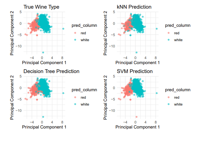
Principal Component Analysis

PCA results demonstrating data distribution and class separation
Optimal Cluster Analysis

Elbow method analysis for determining the optimal number of clusters
Silhouette Analysis

Silhouette analysis validating cluster quality and separation
K-means Clustering Results

K-means clustering results showing final cluster assignments and centroids
Hierarchical Clustering Analysis

Hierarchical clustering dendrogram showing cluster relationships
Conclusions
This project demonstrated the application of KNN and Random Forest techniques to real-world classification problems using the UCI Glass and Wine datasets. Several key conclusions emerged:
- The choice of classification algorithm should be informed by the nature of the dataset. Random Forest proved more effective for the complex Glass dataset with its overlapping classes and high-dimensional feature space.
- Parameter tuning is crucial for optimal classification performance. The stark difference in optimal k values between datasets (k=1 for Glass vs. k=5 for Wine) highlights the importance of proper cross-validation.
- Feature importance analysis provided valuable insights into the chemical properties that best distinguish different glass and wine types, which could inform future data collection efforts or simplified classification models.
- The Wine dataset, with its well-separated classes, was considerably easier to classify than the Glass dataset, yielding high accuracy regardless of the classification method used.
- Ensemble methods like Random Forest offer robustness against noise and outliers, making them particularly valuable for real-world applications with messy data.
Limitations: The relatively small size of both datasets limits the generalizability of the findings. Additionally, more advanced feature engineering techniques could potentially improve classification accuracy further.
Reflection
This project deepened my understanding of classification algorithms and their practical application. Working with real-world datasets helped me appreciate the challenges of handling noisy, imperfect data and the importance of proper preprocessing and parameter tuning.
I found the contrast between the two datasets particularly educational. The Wine dataset, with its well-separated classes, reinforced textbook principles about classification. In contrast, the Glass dataset, with its overlapping classes and uneven distribution, presented real-world complexity that required more sophisticated approaches.
The implementation of cross-validation was essential for obtaining reliable performance estimates, especially for the smaller Wine dataset. This reinforced the statistical foundations of machine learning and the importance of robust evaluation methods.
Through this project, I gained practical experience in implementing and comparing different classification methods, analyzing feature importance, and interpreting model results. These skills are directly transferable to real-world data science and analytics problems where classification is required.
Download Full Report
Interested in the complete analysis and R code implementation? Download the full PDF report below.
Download PDF Report